Kexing Ying's website

kexing.ying@epfl.ch

Last updated Aug. 2026

Contents

08 Aug. 2026. Regression and Wiener Chaos

Suppose \(X \sim \mathcal{N}(0,1)\) and let \(h_k(x) = \frac{H_k(x)}{\sqrt{k!}}\) be the normalised Hermite polynomials, so that \(\mathbb{E}[h_j(X)h_k(X)] = \mathbf{1}_{\{j=k\}}\). Then, for any \(Y \in L^2\), the regression function admits the Wiener chaos expansion \begin{equation} \mathbb{E}[Y \mid X] = \sum_{k=0}^\infty a_k h_k(X), \qquad a_k = \mathbb{E}[Yh_k(X)]. \end{equation} Indeed, the first identity is simply the orthogonal decomposition of \(L^2(\sigma(X))\), while the second follows from \[\mathbb{E}[\mathbb{E}[Y \mid X]h_k(X)] = \mathbb{E}[Yh_k(X)].\] In particular, linear regression corresponds exactly to keeping only the zeroth and first chaos.

This gives a simple test for whether the regression function is linear. Suppose a priori that \begin{equation} \mathbb{E}[Y \mid X] \in \bigoplus_{k=0}^K \mathcal{H}_k(X) = \operatorname{span}\{h_0(X),\ldots,h_K(X)\}. \end{equation} Then, the null hypothesis ``\(H_0 : \mathbb{E}[Y \mid X]\) is linear in \(X\)'' holds if and only if \(a_2 = \cdots = a_K = 0\). Given iid observations \((X_i,Y_i)_{i=1}^n\), we define \[\hat a_k = \frac{1}{n}\sum_{i=1}^n Y_i h_k(X_i), \qquad \hat a = (\hat a_2, \ldots, \hat a_K)^\top.\] Writing \(Z_i=(h_2(X_i),\ldots,h_K(X_i))^\top\), the multivariate CLT gives under \(H_0\) \[\sqrt{n}\hat a \implies \mathcal{N}(0,\Sigma), \qquad \Sigma = \operatorname{Cov}(YZ).\] Thus, with \(\hat\Sigma\) the empirical covariance of \(Y_iZ_i\), \begin{equation} T_n = n \hat a^\top \hat\Sigma^{-1}\hat a \implies \chi^2_{K-1}. \end{equation} Hence, large values of \(T_n\) give evidence against linearity of the regression function. Without the finite chaos assumption, the same statistic tests only that the first \(K\) nonlinear chaos coefficients vanish, and instead one can let \(K=K_n \to \infty\) suitably slowly to obtain an omnibus series test.

We can also construct a related test for joint Gaussianity. Suppose now that \(X,Y\) are centred with unit variance and \(X\) is Gaussian. If \((X,Y)\) are jointly Gaussian with \(\rho=\mathbb{E}[XY]\), then \begin{equation}\label{eq:gaussian-hermite-moments} \mathbb{E}[h_j(X)h_k(Y)] = \mathbf{1}_{\{j=k\}}\rho^k. \end{equation} Indeed, this follows by expanding the Gaussian generating function \[\mathbb{E}\left[e^{tX-t^2/2}e^{sY-s^2/2}\right] = e^{\rho st}.\] Thus, joint Gaussianity imposes a collection of moment restrictions on all Hermite chaos levels, whereas the linear regression test above only considers the restrictions involving the first chaos of \(Y\).

For example, fixing \(K\), we may estimate \[c_{jk} = \mathbb{E}[h_j(X)h_k(Y)] -\mathbf{1}_{\{j=k\}}\rho^k\] for \(0\le j,k\le K\), replacing \(\rho\) by \(\hat\rho=n^{-1}\sum_i X_iY_i\). Collecting any non-redundant collection of these restrictions into a vector \(\hat c\), the multivariate CLT and delta method give under joint Gaussianity \[\sqrt{n}\hat c \implies \mathcal{N}(0, V).\] Consequently, \begin{equation} G_n = n\hat c^\top \hat V^{-1}\hat c \implies \chi^2_q, \end{equation} where \(q\) is the number of restrictions and \(\hat V\) is a consistent estimator of the asymptotic covariance (accounting for the estimation of \(\rho\)). Large values of \(G_n\) therefore allows us to reject joint Gaussianity.

28 Jun. 2026. Some notes on the Greeks for convex payoffs

For an option with payoff \(V(T, S_T) = \Phi(S_T)\) at maturity \(T\), one can immediately observe the sign of some of the Greeks if \(\Phi\) is convex or concave. In this note, we will assume that \(\Phi\) is convex (e.g. the vanilla options) and that we are working with the Black-Scholes model. Throughout, we work with respect to the risk neutral measure \(\mathbb{Q}\) and denote \(S\) the underlying asset price, i.e. \[\mathrm{d} S_t = r S_t \mathrm{d} t + \sigma S_t \mathrm{d} W_t, \quad S_0 = S_0.\]

We can easily determine the sign of the Vega \(\mathcal{V} = \partial_\sigma V\). Indeed, suppose we have two volatilities \(\sigma_1 < \sigma_2\) and denote \(S^\sigma\) the underlying asset price with volatility \(\sigma\). Then, we have by the conditional Jensen's inequality that \begin{align*} \mathbf{E}[\Phi(S^{\sigma_1}_T)] & = \mathbf{E}[\Phi(S_0 e^{-rT} \mathcal{E}(\sigma_1 W)_T)] = \mathbf{E}[\Phi(S_0 e^{-rT} \mathcal{E}(W)_{\sigma_1^2 T})]\\ & \le \mathbf{E}[\Phi(S_0 e^{-rT} \mathbf{E}[\mathcal{E}(W)_{\sigma_2^2 T} \mid \mathcal{F}_{\sigma_1^2 T}])]\\ & = \mathbf{E}[\Phi(S_0 e^{-rT} \mathcal{E}(W)_{\sigma_2^2 T})] = \mathbf{E}[\Phi(S^{\sigma_2}_T)]. \end{align*} Hence, we have shown that \(V\) is increasing in \(\sigma\) and thus \(\mathcal{V} \ge 0\) for convex payoffs.

Now, we will show that the Gamma \(\Gamma = \partial_{S_0}^2 V\) is similarly non-negative for convex payoffs. To this end, it suffices to show that the map \(S \mapsto V(0, S)\) is convex. Indeed, fixing \(\lambda \in [0, 1]\) and \(s_1, s_2 > 0\), we have that \begin{align*} & V(0, \lambda s_1 + (1 - \lambda) s_2) = e^{-rT}\mathbf{E}[\Phi((\lambda s_1 + (1 - \lambda) s_2) e^{rT} \mathcal{E}(\sigma W)_T)]\\ =\ & e^{-rT}\mathbf{E}[\Phi(\lambda s_1 e^{rT} \mathcal{E}(\sigma W)_T + (1 - \lambda) s_2 e^{rT} \mathcal{E}(\sigma W)_T)]\\ \le\ & \lambda e^{-rT}\mathbf{E}[\Phi(s_1 e^{rT} \mathcal{E}(\sigma W)_T)] + (1 - \lambda)e^{-rT} \mathbf{E}[\Phi(s_2 e^{rT} \mathcal{E}(\sigma W)_T)]\\ =\ & \lambda V(0, s_1) + (1 - \lambda) V(0, s_2). \end{align*} This also allows us to conclude an upper bound on the Theta \(\Theta = \partial_t V\). In general, we have that (recall we obtain this by applying Itô's lemma to \(V(t, S_t)\) and enforcing the martingale property after discounting) \begin{equation}\label{eq:BS-PDE} rV = \Theta + \frac{1}{2} \sigma^2 S^2 \Gamma. \end{equation} Thus, \(\Theta = rV - \frac{1}{2} \sigma^2 S^2 \Gamma \le rV\) for convex payoffs and in particular, if \(r = 0\), we have that \(\Theta \le 0\) for convex payoffs.

En passant, we note the Gamma scalping strategy via the Black-Scholes PDE \(\eqref{eq:BS-PDE}\). Gamma scalping essentially consists of a self-financing portfolio \(\Pi_t\) where one long an option and while hedging the Delta of said option. Namely, \(\Pi_t = V(t, S_t) - \Delta S_t + B_t\) where \(B_t\) is the position in the risk free asset for balancing. Then, assuming \(r = 0\), we have by \(\eqref{eq:BS-PDE}\) that \(\Theta = -\frac{1}{2} \sigma_{\mathrm{imp}}^2 S^2 \Gamma\) where \(\sigma_{\mathrm{imp}}\) is the implied volatility of the option (i.e. obtained by inverting the Black-Scholes formula). Now, assuming \(r = 0\), we have that \[\mathrm{d} \Pi_t = \Theta_t \mathrm{d} t + \frac{1}{2} \sigma^2_{\mathrm{real}, t} S^2_t \Gamma_t \mathrm{d} t + \Delta_t \mathrm{d} S_t - \Delta_t \mathrm{d} S_t = \frac{1}{2} S_t^2 \Gamma_t (\sigma^2_{\mathrm{real}, t} - \sigma^2_{\mathrm{imp}}) \mathrm{d} t.\] Consequently, for convex payout functions, as we had demonstrated that \(\Gamma \ge 0\), if the realized volatility is greater than the implied volatility, then \(\mathrm{d} \Pi_t \ge 0\) and the Gamma scalping strategy is profitable.

We also mention that the Delta \(\Delta = \partial_{S_0} V\) is non-negative for monotone payoffs (and non-positive for decreasing payoffs). Indeed, this is immediate from the fact that \[V(0, s_1) = e^{-rT} \mathbf{E}[\Phi(s_1 e^{rT} \mathcal{E}(\sigma W)_T)] \le e^{-rT} \mathbf{E}[\Phi(s_2 e^{rT} \mathcal{E}(\sigma W)_T)] = V(0, s_2)\] for \(s_1 \le s_2\) if \(\Phi\) is increasing.

Vanilla options

In the special case of the vanilla call option, we have the Black-Scholes formula \[C_0 = S_0 \mathcal{N}(d_+) - e^{-rT} K\mathcal{N}(d_-)\] with \(d_\pm = \frac{\log(S_0 / K) + (r \pm \frac{1}{2} \sigma^2)T}{\sigma \sqrt{T}}\) and \(\mathcal{N}\) the CDF of the standard normal distribution. From this, we immediately (by Delta hedging) have that \(\Delta = \mathcal{N}(d_+)\). Alternatively, we can differentiate directly the vanilla call option price to obtain \[\Delta = \mathbf{E}\left[\frac{\tilde S_T}{S_0} \mathbf{1}_{\{S_T \ge K\}}\right] = \mathcal{N}(d_+)\] where we used the identity \(\mathbf{E}[e^{aZ - \frac{1}{2}a^2} \mathbf{1}_{\{Z \ge b\}}] = \mathcal{N}(a - b)\) for \(Z \sim \mathcal{N}(0, 1)\) (this is a special case of the Cameron-Martin theorem!). From this, one easily also obtain the Delta of the vanilla put option via put-call parity.

Of course, we can differentiate \(\Delta\) to obtain \(\Gamma\). However, one can also obtain \(\Gamma\) directly by considering the following observation. Formally, for an call option \(C\) with strike \(K\) and maturity \(T\), we have that \[\partial^2_K C_0 = e^{-rT}\mathbf{E}[\partial^2_K(S_T - K)^+] = e^{-rT} \mathbf{E}[\delta_K(S_T)] = e^{-rT} f_{S_T}(K)\] where \(f_{S_T}\) is the implied distribution, i.e. the density of \(S_T\) under the risk neutral measure (and as before, so are the expectations). Thus, the map \(K \mapsto C_0(S_0, K)\) is convex (and decreasing from \(S_0\) to 0). On the other hand, by computing directly, it is not difficult to see that \(\partial^2_K C_0 = \left(\frac{S_0}{K}\right)^2\Gamma\) and so, we have the formula \[\Gamma = \frac{K^2}{S_0^2} e^{-rT} f_{S_T}(K).\]

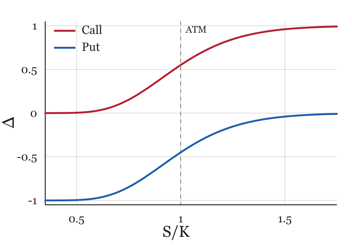
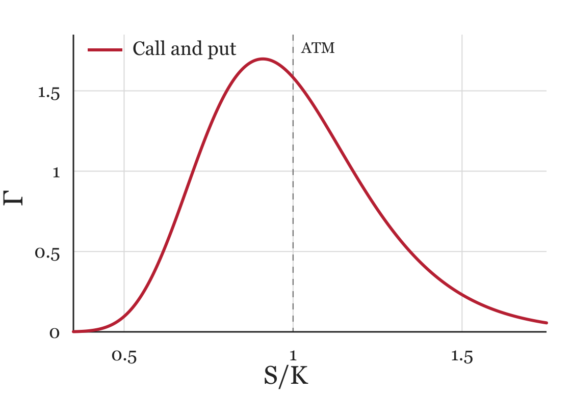
In general, the Delta and Gamma of the vanilla call and put options have a rather characteristic shape as a function of the underlying asset price \(S\) (see the figure below). This is rather useful in practice as it allows one to quickly estimate the Delta and Gamma of linear combinations of vanilla options (e.g. straddle, strangle, call spread, butterfly).

The Greeks via the Malliavin Calculus

Consider an option with payoff \(V(T, S_T) = \mathbf{1}_{\{S_T \ge K\}}\) for some strike \(K\) and maturity \(T\) with \(S\) following the standard Black-Scholes model. We are interested in the Delta of this option. Setting (working wrt the risk neutral measure) \[X_t = \log S_t = \log S_0 + \left(r - \frac{\sigma^2}{2}\right) t + \sigma W_t,\] we have that formally \[\Delta = \partial_{S_0} V(0, S_0) = \partial_{S_0} \mathbf{E}[e^{-rT} \mathbf{1}_{\{S_T \ge K\}}] = \frac{e^{-rT}}{S_0}\mathbf{E}[\delta_{\log K}(X_T)]\] where \(\delta_{\log K}\) is the Dirac delta distribution at \(\log K\). However, the above expression is purely formal and so, we cannot directly use it to compute the Delta (via Monte Carlo simulation for example). Instead, denoting \(\mathcal{D}\) the Malliavin derivative wrt \(W\), we note that \[\mathcal{D}\mathbf{1}_{\{X_T \ge \log K\}} = \delta_{\log K}(X_T) \mathcal{D} X_T = \sigma \delta_{\log K}(X_T) \mathbf{1}_{[0, T]}.\] Thus, we have that \begin{align*} \mathbf{E}[\delta_{\log K}(X_T)] & = \mathbf{E}\left[\langle \delta_{\log K}(X_T), 1\rangle _{L^2([0, T])}\right] = \frac{1}{\sigma}\mathbf{E}\left[\langle \mathcal{D}\mathbf{1}_{\{X_T \ge \log K\}}, 1\rangle _{L^2([0, T])}\right]\\ & = \frac{1}{\sigma}\mathbf{E}[\mathbf{1}_{\{X_T \ge \log K\}} \delta(1)] = \frac{1}{\sigma}\mathbf{E}[\mathbf{1}_{\{S_T \ge K\}} W_T]. \end{align*} Consequently, combining the above, we have that \[\Delta = \frac{e^{-rT}}{\sigma S_0} \mathbf{E}[\mathbf{1}_{\{S_T \ge K\}} W_T].\] This expression is well-defined from which we can compute the Delta via Monte Carlo simulation.

While the above computation relies heavily on the fact that the Dirac delta of the log price \(X_T\) can be expressed as the Malliavin derivative of a well defined random variable, more general payoffs can be handled as well by noting the following integration by parts formula.

Lemma. Assuming \(\Phi\) is weakly differentiable and \(X\) is Malliavin differentiable, we have that \[\mathbf{E}[\Phi'(X)] = \mathbf{E}[\Phi(X) \delta(h)]\] for any \(h\) satisfying \(\langle \mathcal{D}X, h\rangle _{\mathcal{H}} = 1\) a.s.

Proof. Indeed, this follows straightaway as \[\mathbf{E}[\Phi'(X)] = \mathbf{E}[\Phi'(X) \langle \mathcal{D}X, h\rangle _{\mathcal{H}}] = \mathbf{E}[\langle \mathcal{D}\Phi(X), h\rangle _{\mathcal{H}}] = \mathbf{E}[\Phi(X) \delta(h)].\]

□

With this lemma in mind, let us consider the following example. Assume we now have the payoff \(V(T, S_T) = \mathbf{1}_{\{A_T \ge K\}}\) where \(A_T = \frac{1}{T} \int_0^T S_t \mathrm{d} t\) is the average price of the underlying asset. In this case, we have that \[\partial_{S_0} A_T = \frac{1}{T} \int_0^T \partial_{S_0} S_t \mathrm{d} t = \frac{1}{T} \int_0^T \frac{S_t}{S_0} \mathrm{d} t = \frac{A_T}{S_0}\] where in the second equality, we used the fact that \(S_t = S_0 \exp\left(\left(r - \frac{\sigma^2}{2}\right) t + \sigma W_t\right)\). Hence, we have that \[\Delta = e^{-rT} \mathbf{E}\left[\delta_{K}(A_T) \frac{A_T}{S_0}\right] = \frac{e^{-rT} K}{S_0}\mathbf{E}[\delta_{K}(A_T)]\] and we are interested in computing \(\mathbf{E}[\delta_{K}(A_T)]\). To this end, using the integration by parts formula, we want to find \(h\) such that \(\langle \mathcal{D}A_T, h\rangle _{L^2([0, T])} = 1\). One simple choice it to take \(h\) to be constant in time. In this case, we have that \begin{align*} \langle \mathcal{D}A_T, h\rangle _{L^2([0, T])} & = h \int_0^T \mathcal{D}_t A_T \mathrm{d} t = \frac{h}{T} \int_0^T \int_0^T \mathcal{D}_t S_u \mathrm{d} u \mathrm{d} t\\ & = \frac{h}{T} \int_0^T \int_0^T \sigma S_u \mathbf{1}_{[0, u]}(t) \mathrm{d} u \mathrm{d} t = \frac{\sigma h}{T} \int_0^T t S_t \mathrm{d} t. \end{align*} Thus, taking \(h = \left(\frac{\sigma}{T} \int_0^T t S_t \mathrm{d} t\right)^{-1}\) suffices and it remains to compute \(\delta(h)\). For this, since \(h\) is a constant random variable, we have that \(\delta(h) = h W_T - \langle \mathcal{D}h, 1\rangle _{L^2([0, T])}\) where \[\mathcal{D}_u h = - \frac{\sigma h^2}{T} \int_0^T t \mathcal{D}_u S_t \mathrm{d} t = - \frac{\sigma^2 h^2}{T} \int_0^T t S_t \mathbf{1}_{[0, t]}(u) \mathrm{d} t.\] Hence, \[\langle \mathcal{D}h, 1\rangle _{L^2([0, T])} = - \frac{\sigma^2 h^2}{T} \int_0^T t^2 S_t \mathrm{d} t = - \frac{T \int_0^T t^2 S_t \mathrm{d} t}{\left(\int_0^T t S_t \mathrm{d} t\right)^2}.\] Combining the above, we find \[\Delta = \frac{e^{-rT} K}{S_0}\mathbf{E}\left[\mathbf{1}_{A_T \ge K} \left(\frac{W_T}{\frac{\sigma}{T} \int_0^T t S_t \mathrm{d} t} + \frac{T \int_0^T t^2 S_t \mathrm{d} t}{\left(\int_0^T t S_t \mathrm{d} t\right)^2}\right)\right].\]

22 Jun. 2026.   Some notes on cumulants

Cumulants and independence

The cumulants provide a direct description of the independence of random variables and in particular, explains why, in the case of Gaussian random variables, the covariance is enough to describe their independence.

Straightaway from the definition of the cumulants, as for any random variables \(X\) and \(Y\), \(X\) and \(Y\) are independent if and only if their joint moment generating function factorizes, i.e. their joint cumulant generating function \(K_{X, Y}(t, s)\) satisfies \[K_{X, Y}(t, s) = K_X(t) + K_Y(s).\] Thus, writing out the Taylor expansions \begin{align*} K_{X, Y}(t, s) & = \sum_{m, n \ge 0} \frac{\kappa_{m, n}(X, Y)}{m! n!} t^m s^n\\ K_X(t) + K_Y(s) & = \sum_{m, n \ge 0} \left(\frac{\kappa_m(X)}{m!} t^m + \frac{\kappa_n(Y)}{n!} s^n\right) \end{align*} we match the coefficients from which we conclude that \(X\) and \(Y\) are independent if and only if \[\kappa_{m, n}(X, Y) = 0 \quad \text{for all } m, n \ge 1.\] Namely, we require that all mixed cumulants must vanish. From this, we immediately see that for \((X, Y)\) jointly Gaussian, the covariance is enough to describe their independence. Indeed, for Gaussians, all cumulants of order strictly higher than 2 vanish and so, \(\kappa_{m, n}(X, Y) = 0\) automatically for all \(m + n \ge 3\). Thus, the only non-trivial mixed cumulant is \(\kappa_{1, 1}(X, Y) = \mathrm{Cov}(X, Y)\) and so, if \(\mathrm{Cov}(X, Y) = 0\), we have that \(X\) and \(Y\) are independent.

The diagram formula

The cumulants are useful in computing the moments of a random variable. In particular, for a family of random variable \((X_i)_{i \in A}\), we have that \[\mathbf{E}\left[\prod_{i \in A} X_i\right] = \sum_{\Delta \in \mathcal{P}(A)} \prod_{B \in \Delta} \mathbf{E}_c\left[\prod_{i \in B} X_i\right]\] where \(\mathcal{P}(A)\) is the set of all partitions of \(A\) and \(\mathbf{E}_c\) is the cumulant. For instance, writing \(\kappa_j := \mathbf{E}_c[X^j]\), a block containing \(j\) points represents the factor \(\kappa_j\), and the sixth moment is computed by the diagram formula as \[\begin{aligned} \mathbf{E}[X^6] =\ & \kappa_6 + 6\kappa_5\kappa_1 + 15\kappa_4\kappa_2 + 10\kappa_3^2 + 15\kappa_4\kappa_1^2 + 60\kappa_3\kappa_2\kappa_1 \\ &+ 15\kappa_2^3 + 20\kappa_3\kappa_1^3 + 45\kappa_2^2\kappa_1^2 + 15\kappa_2\kappa_1^4 + \kappa_1^6 . \end{aligned}\] Hence, in the case where \(X\) has well-known cumulants (e.g. Gaussian or Poisson), we can easily compute its moments by counting the number of possible partitions and adding their corresponding cumulants together.

Cumulants and the CLT

Consider a sequence of iid random variables \((X_i)_{i=1}^\infty\) for which we take the usual CLT scaling \(S_n := \frac{1}{\sqrt{n}} \sum_{i=1}^n X_i\). Assuming all cumulants of \(X_i\) are finite, we immediately obtain the CLT by looking at the cumulants of \(S_n\). Indeed, as \[\kappa_k(S_n) = \frac{1}{n^{k / 2}} \sum_{i=1}^n \kappa_k(X_i) = n^{1 - \frac{k}{2}}\kappa_k(X_1),\] we immediately have that \(\kappa_k(S_n) \to 0\) for all \(k \ge 3\). Thus, as the Gaussian is uniquely characterized by the fact that all its cumulants of order higher than 2 vanish, we have that \(S_n\) converges in distribution to a Gaussian. Moreover, we can guess that the rate of convergence is \(O(n^{-1/2})\) in some suitable metric (e.g. the Wasserstein distance) as \(\kappa_3(S_n) = O(n^{-1/2})\) with higher order cumulants decaying even faster.

25 May. 2026.   The Ornstein-Uhlenbeck Process and the Dickey-Fuller Test

Let us consider the Ornstein-Uhlenbeck (OU) process \(X\) on \(\mathbb{R}\) defined by the SDE \begin{equation} \mathrm{d} X_t = -\theta X_t \mathrm{d} t + \sigma \mathrm{d} W_t \end{equation} for some \(\theta, \sigma > 0\) and \(W\) a standard Brownian motion. By the variation of constants formula (a.k.a. the Duhamel principle, a.k.a. the mild formulation), we have that \(L = - \theta\) and \(P_t = e^{tL} = e^{-\theta t}\). Thus, we have the solution \[X_t = e^{-\theta t} X_0 + \sigma \int_0^t e^{-\theta (t-s)} \mathrm{d} W_s.\]

Invariant measure and moments

Straight away from this, we can read off that if \(X_0 \sim \sigma \int_{-\infty}^0 e^{\theta s} \mathrm{d} W_s\) with \(W\) a two-sided Brownian motion, then \(X\) is stationary. However, suppose we instead know that the OU process has Gaussian invariant measure \(\mu\), we can also figure out its variance by the following argument (\(\mu\) is clearly centered).

Denoting \(\mathcal{L} = \frac{\sigma^2}{2} \Delta -\theta x \nabla\) now the generator of the OU process, we have by Fokker-Planck that \(\mathcal{L}^* \mu = 0\). Namely, for any test function \(f\), we have that \(\mathbf{E}_\mu[\mathcal{L}f] = 0\). Thus, taking \(f(x) = x^2\), we have that \begin{equation} 0 = \mathbf{E}_\mu[\mathcal{L}f] = \mathbf{E}_\mu[\sigma^2 - 2\theta x^2] = \sigma^2 - 2\theta \mathbf{E}_\mu[x^2]. \end{equation} Thus, we have \(\mathbf{E}_\mu[x^2] = \frac{\sigma^2}{2\theta}\) as expected. Of course, replacing \(x^2\) with any other test functions allows us to obtain other \(\mathbf{E}_\mu[f]\) as well. Namely, suppose we are interested in finding \(\mathbf{E}[f(Z)]\) for \(Z \sim \mathcal{N}(0, 1)\). Then, by setting \(f(x) = xg'(x)\), we have that \(g''(x) = \left(\frac{f(x)}{x}\right)'\) and thus (taking \(\theta = 1\), \(\sigma^2 = 2\)), \[\mathbf{E}[f(Z)] = \mathbf{E}[(x^{-1}f(x))'|_{x = Z}].\] As an example, suppose \(f(x) = |x|^3\) (of course, this can also be found by directly computing the integral). Then, \(x^{-1}f(x) = x|x|\) which has derivative \(2|x|\). Repeating this one more time, we have \((x^{-1}|x|)' = 2 \delta_0\) and thus, denoting \(p_1\) for the density function of \(Z\), we have that \[\mathbf{E}[|Z|^3] = 2\mathbf{E}[|Z|] = 4 \int \delta_0(x) p_1(x) \mathrm{d} x = 4 p_1(0) = 2\sqrt{\frac{2}{\pi}}.\] Moreover, one finds that taking \(f(x) = |x|^{2n + 1}\), we have that \((x^{-1}f(x))' = 2n |x|^{2n - 1}\). Hence, it follows that \(\mathbf{E}[|Z|^{2n + 1}] = 2^n n! \sqrt{\frac{2}{\pi}}\).

Parameter estimation

Suppose we observe one trajectory of the OU process. We can estimate \(\theta\) as follows. By approximating the SDE by the Euler scheme, we have that for small \(h\), that \begin{equation}\label{eq:euler-scheme} X_{t + h} - X_{t} \approx - \theta h X_{t} + \sigma \sqrt{h} Z_i. \end{equation} Thus, we can estimate \(\theta\) by regressing \(X_{t + h} - X_{t}\) against \(X_t\) (with the intercept fixed to be zero). Writing out the OLS estimator, we have that \begin{equation}\label{eq:hat-theta} \hat{\theta} = -\frac{\sum_{i=1}^n X_{t_i}(X_{t_i + h} - X_{t_i})}{h \sum_{i=1}^n X_{t_i}^2} \to -\frac{\int_0^T X_t \mathrm{d} X_t}{\int_0^T X_t^2 \mathrm{d} t} \end{equation} as \(h \to 0\) and \(n \to \infty\) with \(nh = T\) fixed. Note that this convergence is only in probability (c.f. rough path theory).

Alternatively, in this case, since we know the exact formula for the solution of the OU process, we have that \[X_{t + h} = e^{-\theta h} X_t + \sigma \int_t^{t + h} e^{-\theta(t + h - s)} \mathrm{d} W_s.\] Namely, \((X_{kh})_{k = 1}^N\) is an autoregressive model from which we can estimate \(\theta\) via the AR regression.

Another useful method in estimating properties of the invariant measure is to use the Birkhoff ergodic theorem. In particular, for the OU process, by looking at the covariance function, we have that \(X_t\) is mixing and so, is ergodic. Hence, by the mean ergodic theorem, we have that for any \(f \in L^1(\mu)\), \begin{equation} \frac{1}{T} \int_0^T f(X_t) \mathrm{d} t \to \mathbf{E}_\mu[f] \quad \text{as } T \to \infty \end{equation} almost surely. Thus, by taking a time average of \(f(X_t)\) for some test function \(f\), we can estimate \(\mathbf{E}_\mu[f]\) as well. As an example, suppose we are interested in estimating the tail of the invariant measure \(\mu\). In this case, taking \(f(x) = \mathbf{1}_{\{x > R\}}\), we have that \begin{equation} \frac{1}{T} \int_0^T \mathbf{1}_{\{X_t > R\}} \mathrm{d} t \to \mathbf{E}_\mu[\mathbf{1}_{\{x > R\}}] = \mu(R, \infty) \end{equation} as \(T \to \infty\) almost surely. Note that, to show that the OU process is mixing, we can compute the covariance function explicitly. In particular, for any \(t, s \ge 0\), we have that \begin{equation} \mathrm{Cov}(X_t, X_{t + s}) = \frac{\sigma^2}{2\theta} e^{-\theta s} \to 0 \end{equation} and thus, \(X\) is mixing as claimed.

However, we note that in this case of the OU process, ergodicity cannot directly provide us with an estimate for \(\theta\). Indeed, as the right hand side depends only on the invariant measure \(\mu \sim \mathcal{N}(0, \sigma^2 / (2\theta))\), one can only estimate the parameter \(\sigma^2 / (2\theta)\).

We are interested in the behavior of the OLS estimator \(\eqref{eq:hat-theta}\). We remark that, unlike for simple linear regression models, the samples we use for regression \((-h X_{t_i}, X_{t_i + h} - X_{t_i})_{i}\) is clearly not independent, and so, we cannot directly apply the SLLN to obtain consistency of the estimator. Instead, to justify the convergence of the OLS estimator \(\hat \theta\), we can use the martingale convergence theorems. In general, consider the following set up. Suppose we have \((X_i)\) an ergodic process and \[Y_i = \beta X_i + \epsilon_i\] with \(\mathbf{E}[\epsilon_i \mid X_i] = 0\). Then, we have that the estimate \[\hat \beta = \frac{\sum_{i = 1}^n X_i Y_i}{\sum_{i = 1}^n X_i^2} = \beta + \frac{\sum_{i = 1}^n X_i \epsilon_i}{\sum_{i = 1}^n X_i^2}.\] Hence, as \(\mathbf{E}[\epsilon_i \mid X_i] = 0\), we have that \(\frac{1}{n}\sum_{i = 1}^n X_i \epsilon_i\) is a UI martingale which converges to 0 a.s. and in \(L^p\). On the other hand, by the ergodic theorem, the denominator \(\frac{1}{n}\sum_{i = 1}^n X_i^2 \to \mathbf{E}_\mu[x^2]\) as \(n \to \infty\). Thus, we have that \(\hat \beta \to \beta\) as claimed. In statistical language, we say that \(\hat \beta\) is strongly consistent.

Let us now consider the fluctuations of the estimator \(\eqref{eq:hat-theta}\). We define \[\hat \theta - \theta = \frac{- \sigma \int_0^T X_s \mathrm{d} B_s}{\int_0^T X_s^2 \mathrm{d} s} =: -\sigma \frac{M_T}{\langle M\rangle _T}.\] While this fraction looks nice at a glance, with a martingale in the numerator and its quadratic variation in its denominator, it doesn't seem easily boundable. Instead, I'll provide some back of the envelope calculations. Applying Itô's formula, we obtain \[\mathrm{d} (X_t^2) = - 2 \theta \mathrm{d} \langle M\rangle _t + 2 \sigma \mathrm{d} M_t + \sigma^2 t,\] and so, \[\sigma \frac{M_T}{\langle M\rangle _T} = \theta + \frac{X_T^2 - X_0^T - \sigma^2 T}{2 \langle M\rangle _T}.\] Since the OU process is stationary, we expect that \(X_t\) has typical size \(O(1)\). On the other hand, by the ergodic theorem \(\frac{1}{T}\langle M\rangle _T \sim \mathbf{E}_\mu[x^2] = \frac{\sigma^2}{2\theta}\). So, assuming some CLT type fluctuations, we have that \[\frac{1}{\sqrt{T}}\left(\langle M\rangle _T - \frac{\sigma^2 T}{2\theta}\right) \sim O(1)\] or equivalently, \[\frac{1}{\langle M\rangle _T} \sim \left(\frac{\sigma^2 T}{2\theta}\right)^{-1}\left(1 + \frac{1}{\sqrt{T}} + o\left(\frac{1}{\sqrt{T}}\right)\right)^{-1} \sim \frac{2\theta}{\sigma^2 T}\left(1 - \frac{1}{\sqrt{T}} + o\left(\frac{1}{\sqrt{T}}\right)\right)\] and we obtain a rough estimate \[\sigma \frac{M_T}{\langle M\rangle _T} \sim \theta - \frac{\theta(\sigma^2T + O(1))}{\sigma^2 T}\left(1 - \frac{1}{\sqrt{T}} + o\left(\frac{1}{\sqrt{T}}\right)\right) \sim \frac{1}{\sqrt{T}} + o\left(\frac{1}{\sqrt{T}}\right).\] Thus, from this, any possible bias is contained in the higher order terms \(O(T^{-1})\), i.e. the bias (if any) decays faster than the fluctuation.

The Dickey-Fuller Test

The estimator \(\eqref{eq:hat-theta}\) we obtained for the OU process essentially corresponds to the classical Dickey-Fuller test (DF). We recall that the DF test is a hypothesis test for an \(\mathrm{AR}(1)\) process in which we determine whether or not a process of the form \[x_{t + 1} = \rho x_t + \sigma \epsilon_t, \qquad \epsilon_t \sim \mathcal{N}(0, 1) \text{ iid.}\] is a random walk (or is it stationary), i.e. \(H_0 : \rho = 1\). Comparing with the Euler scheme \(\eqref{eq:euler-scheme}\), namely, by writing \(\Delta x_t = (\rho - 1) x_t + \epsilon_t\), we obtain the same scheme as the discretized OU process and we can regress \(x_t\) against \(\Delta x_t\). In particular, under \(H_0\), we have the OLS estimator for \(\rho - 1\) \[\hat \beta = \frac{\int_0^T x_t \mathrm{d} x_t}{\int_0^T x_t^2 \mathrm{d} t} = \frac{T\sigma^2 \int_0^1 \left(\frac{x_{Tt}}{\sigma\sqrt{T}}\right) \mathrm{d} \left(\frac{x_{Tt}}{\sigma\sqrt{T}}\right)}{T^2 \sigma^2\int_0^1 \left(\frac{x_{Tt}}{\sigma\sqrt{T}}\right)^2 \mathrm{d} t} \stackrel{T \gg 1}{\implies} \frac{1}{T} \frac{\int_0^1 B_t \mathrm{d} B_t}{\int_0^1 B_t^2 \mathrm{d} t} = \frac{1}{T}\frac{B_1^2 - 1}{2 \int_0^1 B_t^2 \mathrm{d} t}.\] Thus, under \(H_0\), \(\hat \beta\) has known non-Gaussian fluctuations for which we can perform statistical tests.

We remark that, from this, we also observe that \(\hat \beta\) does not have the CLT scaling but is instead super diffusive. This is in contrast to the usual OLS estimator (i.e. with iid samples) in which we have that the standard CLT scaling with Gaussian fluctuations. We also contrast this scaling with the one we obtained for the OU process (also CLT scaling). Indeed, this directly corresponds to the scaling one obtains in the case where we reject the null-hypothesis and instead assumes stationarity.

Note that, the above test using \(T \hat \beta\) is not what people usually refer to as the Dickey-Fuller test. Instead, DF usually refers to performing a statistical test with respect to \(\tau := \hat \beta / \mathrm{SE}(\hat \beta)\) with \(\mathrm{SE}(\hat \beta) = \hat \sigma (\sqrt{\sum x_i^2})^{-1}\) where \(\hat \sigma^2\) is the sample variance. Here \(\tau\) is known as the OLS \(t\)-statistic (which does not follow the student \(t\)-distribution) and a similar analysis as above shows that \[\tau = \frac{\hat \beta}{\mathrm{SE}(\hat \beta)} \sim \frac{B_1^2 - 1}{2 \left(\int_0^1 B_t^2 \mathrm{d} t\right)^{1 / 2}}\] in the \(T \to \infty\) limit.

In the case that the white noise \(\epsilon_t\) is replaced by a fractional Gaussian noise \(\epsilon^H_t\), a similar convergence occurs with a phase transition at \(H = 1 / 2\).

Theorem. Let \((x_t)\) be the fractional random walk \(x_{t + 1} = x_t + \epsilon_t^H, \qquad x_0 = 0\) driven by a stationary fGn of Hurst parameter \(H \in (0, 1)\). Then, as \(T \to \infty\),

\(\bullet\) if \(H > 1/2\), \(\displaystyle T \hat\beta_T \implies \frac{(B^H_1)^2}{2 \int_0^1 (B^H_s)^2 \mathrm{d} s}\);

\(\bullet\) if \(H < 1/2\), \(\displaystyle T^{2 H} \hat\beta_T \implies \frac{-1}{2 \int_0^1 (B^H_s)^2 \mathrm{d} s}\). where \(B^H\) is a fractional Brownian motion of Hurst parameter \(H\).

The proof of this follows directly by analysing the (discrete) quadratic variation of the fGn for which the two regimes \(H > 1/2\) and \(H < 1/2\) correspond to the cases of vanishing and diverging quadratic variations.

19 May. 2026.   RKHS in statistics and the Cameron-Martin space

Suppose now \(X\) is a Gaussian random variable on some Banach space \(\mathcal{B}\) with law \(\mu\). We recall that the Cameron-Martin space \(\mathcal{H}_\mu\) of \(\mu\) is defined as the closure (with respect to the Cameron-Martin norm) of the pre-Cameron-Martin space \[ \mathcal{H}_{\mu}^\circ = \left\{ x \in \mathcal{B} : \exists\, x^{*} \in \mathcal{B}^*,\ l(x) = C_\mu(l, x^{*})\ \forall\, l \in \mathcal{B}^{*} \right\} = C_\mu(\mathcal{B}^*) \] where in the latter equality we identify \(C_\mu : \mathcal{B}^* \to \mathcal{B}\) by \(C_\mu l = \int l(x) x\, \mu(\mathrm{d} x)\) with the integral understood in the Bochner sense.

We show that the Cameron-Martin space is exactly the RKHS (in the statistician's sense) associated to the kernel \(k(h, k) = C_\mu(h, k) = \int h(x) k(x)\, \mu(\mathrm{d} x)\) (to be more precise, the RKHS of \(k\) is the canonical identification of \(\mathcal{H}_\mu\) in \(\mathcal{B}^{**}\)). Note that the RKHS here is different from the RKHS in Hairer's notes on Malliavin calculus¹ which is instead the \(L^2(\mu)\)-closure of \(\mathcal{B}^*\).

Recall that the RKHS \(\mathcal{H}\) associated to a reproducing kernel \(k : \mathcal{X} \times \mathcal{X} \to \mathbb{R}\) is a Hilbert space of functions \(f : \mathcal{X} \to \mathbb{R}\) such that \(k(x, \cdot) =: k_x \in \mathcal{H}\) for all \(x\) and \[ \langle f, k(x, \cdot) \rangle_{\mathcal{H}} = f(x). \] In general, the RKHS \(\mathcal{H}\) is canonically defined by \(\mathcal{H} = \overline{\mathcal{H}^\circ} = \overline{\langle k(x, \cdot) : x \in \mathcal{X} \rangle}^\mathcal{H}\) with the closure taken with respect to the topology generated by the inner product \[ \left\langle \sum_i \alpha_i k(x_i, \cdot), \sum_j \beta_j k(x_j, \cdot) \right\rangle_\mathcal{H} = \sum_{i, j} \alpha_i \beta_j k(x_i, x_j). \]

In this case, \(\mathcal{X} = \mathcal{B}^*\) and \(\mathcal{H} = \mathcal{H}_\mu\) with the canonical identification \(x \in \mathcal{H}_\mu \subseteq \mathcal{B}^{**}\), \(x: l \mapsto l(x)\). Indeed, in this case, \(k(l, \cdot) = C_\mu l \in \mathcal{H}_\mu^\circ\) and for any \(x \in \mathcal{H}_\mu^\circ\), we have that \[ \langle x, k(l, \cdot) \rangle_\mu = \langle x, C_\mu l \rangle_\mu = C_\mu(x^{*}, l) = l(x) = x(l) \] where we used the fact that \((C_\mu l)^* = l\).

Conversely, suppose we have the reproducing kernel \(k : \mathcal{X} \times \mathcal{X} \to \mathbb{R}\) (recall it is symmetric and positive definite) and its associated RKHS \(\mathcal{H}\). In this case, we consider a isonormal Gaussian process \(W\) on \(\mathcal{H}\) (and its first chaos \(\mathcal{H}_1\) is isomorphic to \(\mathcal{H}\) via the map \(h \mapsto W(h)\)). On the other hand, under some mild regularity assumptions (e.g. via Kolmogorov continuity criterion), there exists a Gaussian measure \(\mu\) on some Banach space \(\mathcal{B} \subseteq \mathbb{R}^\mathcal{H}\) for which the Cameron-Martin space is exactly \(\mathcal{H}_1\). Thus, in this case, the above correspondence between the Cameron-Martin space and the RKHS holds as well.

With this language in mind, viewing \(X\) as an isonormal Gaussian process over an RKHS \(\mathcal{H}\), linear regression corresponds to finding the component of the regression function in the first chaos of \(X\). Namely, taking \(Z_n \in \mathcal{H}_n\) with \(Z_1 = X(h)\) such that \[\mathbf{E}[Y \mid X] = \sum_{n = 1}^\infty Z_n =: Z \in L^2 = \bigoplus_{n=1}^\infty \mathcal{H}_n,\] linear regression corresponds to estimating \(h \in \mathcal{H}\) (or equivalently, estimating \(DZ\) - the Malliavin derivative of \(Z\) against \(X\)).

1. https://www.hairer.org/notes/Malliavin.pdf ↩

05 Mar. 2026.   Recurrence of planar Brownian motion

I first saw the recurrence (in small balls) property of planar Brownian motion a couple years ago during the Advanced Probability course offered by Part III. The proof I saw was of course (I believe) the standard approach in which one uses the fact that the Brownian motion composed with any harmonic function remains to be a martingale. In particular, by using the logarithm, this fact (and the optional stopping theorem) allows us to easily compute the probability that the Brownian motion hits a small ball before hitting a larger one. Thus, by taking the radius of the larger ball to infinity, we finds that the Brownian motion hits the small ball with probability one.

This problem came up again recently during the exercise session of the Random Geometry course offered here at EPFL and, in an attempt at avoiding martingale techniques, Colin Piernot and I (mostly Colin) found a clever proof of this the sketch of which I would like to share here.

Theorem. Let \(B_t\) be a complex Brownian motion and \(z\) be a point in the complex plane. Then, for any \(\epsilon > 0\), we have that \[\mathbb{P}(|B_t - z| < \epsilon \text{ i.o.}) = 1.\]

Proof. By translation, we my assume without loss of generality that \(z = 0\) and the Brownian motions starts at \(1\).

Let us define the following continuous time random walk \(X_t\) on \(\mathbb{Z}\): Defining \(\tau_0 = 0\) \[\tau_{n + 1} := \inf\{t > \tau_n : |B_t| \in 2^{\mathbb{Z}} \setminus \{|B_{\tau_n}|\}\}\] we set \(X_t = \log_2 |B_{\tau_n}|\) whenever \(t \in [\tau_n, \tau_{n + 1})\). Namely, \(X_t\) is the continuous time random walk which moves to \(n\) whenever the Brownian motion hits the circle of radius \(2^n\). Thus, as hitting the \(\epsilon\)-ball centered at the origin corresponds to \(X_t\) hitting \(n\) for any \(n \in \mathbb{Z}\) satisfying \(2^n < \epsilon\), it follows that the conclusion holds if we can show that \(X_t\) is symmetric (and so, is recurrent).

Straightaway, by scaling invariance and the strong Markov property, it suffices to show that \[\mathbb{P}(X_{\tau_1} = 0) = \mathbb{P}(X_{\tau_1} = 2) = \frac{1}{2}.\] Namely, we need to show that \(B_t\) hits the circle of radius \(1/2\) before the circle of radius \(2\) with probability \(1/2\). However, this is clear as, the map \[f : A \to A : z \mapsto \frac{1}{z}\] with \(A\) being the annulus \(\{z \in \mathbb{C} : 1/2 \le |z| \le 2\}\) is conformal. Thus, as \(f\) maps the boundary \(\{|z| = 2\}\) to \(\{|z| = 1/2\}\) and \(f(B_t)\) is also a Brownian motion starting at 1 (by the conformal invariance of Brownian motion), the conclusion holds by symmetry.

□

Interestingly (or maybe not so considering the topic of the course), this type of argument also appeared later in the Random Geometry course in the probabilistic proof of the Picards little theorem. There, starting with the Brownian motion's image over a conformal map, one similarly constructs a random walk on \(\mathbb{Z}^2\) (albeit here the construction is much more complicated with a lot of nuances. In particular, here the random walk is associated with the winding number of the trace quotiented by an equivalence relation in order to obtain integrability). Then, by showing that this radom walk is transient, one is able to conclude the theorem.

19 Oct. 2024.   Disjointness and Mutually Singular

For an ordered set \((X, \le)\), we say \(x, y \in X\) are disjoint if for any \(z \le x\) and \(z \le y\), we have that \(z = \perp\). Rémy Degenne observed that, in the case of \(\sigma\)-finite measures, the notion of mutually singular is equivalent to disjointness. He then asked whether or not this fact generalizes to arbitrary measures (Rémy's proof used the Radon-Nikodym derivative and consequently relies on \(\sigma\)-finiteness). In this short note, we provide an elementary proof of this equivalence without assuming \(\sigma\)-finiteness.

For a measurable space \((X, \Sigma)\) and two measures \(\mu, \nu\) on \((X, \Sigma)\), we define the measure \(\mu \wedge \nu\) by \[(\mu \wedge \nu)(S) = \inf \{\mu(S \cap T) + \nu(S \cap T^c) \mid T \in \Sigma\}.\] It is a standard exercise to check that this is indeed a bona-fide measure and that \(\mu \wedge \nu \le \mu\) and \(\mu \wedge \nu \le \nu\).

Fixing \(\epsilon > 0\) and \(n \in \mathbb{N}\), as \((\mu \wedge \nu)(X) = 0\), we have by construction that there exists \(S_n^\epsilon \in \Sigma\) such that \[\mu(S_n^\epsilon) + \nu((S_n^\epsilon)^c) \le \epsilon 2^{-n}.\] Thus, denoting \(S^\epsilon = \bigcap_{n \in \mathbb{N}} S_n^\epsilon\), we have that \(\mu(S^\epsilon) = 0\) and \[\nu((S^\epsilon)^c) = \nu\left(\bigcup_{n \in \mathbb{N}} (S_n^\epsilon)^c\right) \le \sum_{n \in \mathbb{N}}\epsilon 2^{-n} = \epsilon.\] Finally, taking \(S = \bigcup_{n \in \mathbb{N}} S^{1 / n}\), \(\mu(S) = 0\) as \(S\) is a countable union of \(\mu\)-null-sets while \[\nu(S^c) = \nu\left(\bigcap_{n \in \mathbb{N}} (S^{1 / n})^c\right) \le \frac{1}{k}\] for all \(k \in \mathbb{N}\) implying that \(\nu(S^c) = 0\). Thus, \(\mu\) and \(\nu\) are mutually singular as required.

15 May. 2024.   An Application of the Cameron-Martin Theorem

The Cameron-Martin theorem provides a characterization of the Gaussian measure on infinite dimensional spaces. In this entry, I'll record an application of this theorem in the context of obtaining a maximal inequality for Brownian motions.

The Cameron-Martin theorem is the following.

Theorem. Let \(\mu \in \mathcal{M}(X)\) be a Gaussian and denote \(\mathcal{H}_\mu\) for its Cameron-Martin space. For \(h \in X\) denoting \(\tau_h : x \in X \mapsto x + h\), we have that \(\tau_h^* \mu \ll \mu\) if and only if \(h \in \mathcal{H}_\mu\). In this case, \[\frac{d\tau_h^* \mu}{d\mu}(x) = \exp\left(h^*(x) - \frac{1}{2}\|h\|^2_\mu\right).\]

Let \(\mu\) be the Gaussian measure on \(\mathcal{C}([0, 1], \mathbb{R})\) with covariance \(C_\mu(\delta_t, \delta_s) = s \wedge t\). \(\mu\) corresponds to the law of the Brownian motion on \([0, 1]\) and we call it the Wiener measure. We have that \(\mathcal{H}_\mu = H^{1, 2}_0([0, 1])\) - the space of all absolutely continuous functions \(h\) with \(h(0) = 0\) and \(\dot h(s) \in L^2([0, 1])\). Moreover, for \(h \in \mathcal{H}_\mu\), \(h^*(k) = \int_0^1 \dot h(s) \dot k(s) d s\). As this defines a bounded linear functional from \(\mathcal{H}_\mu\), we can almost surely uniquely extend \(h^*\) to a measurable element of \(C_\mu(\delta_t, \delta_s)^*\). To see this, it suffices to check that \[h_t = \delta_t(h) = C_\mu(\delta_t, h^*) = h^*(C_\mu(\delta_t)).\] We see that \[C_\mu(\delta_t)_s = \left(\int \omega \delta_t(\omega) \mu(d \omega)\right)_s = \int \omega_s \omega_t \mu(d \omega) = C_\mu(\delta_t, \delta_s) = s \wedge t.\] Thus, \(\dot{C}_\mu(\delta_t)_s = \mathbb{1}_{[0, t]}(s)\) and hence, \[h^*(C_\mu(\delta_t)) = \int_0^t \dot f_s d s = f_t\] as required.

As an application, the Cameron-Martin theorem allows us to bound the probability that a Brownian motion stays near a given function. In particular, for \(f \in H^{1, 2}_0([0, 1])\), denoting \(\mu_W\) for the Wiener measure, we have that \[\mathbb{P}(|B_t - f|_\infty \le \epsilon) = \tau_{-f}^* \mu_W(\overline B_\epsilon(0)) = e^{-\frac{1}{2}\|f\|^2_{H^{1, 2}_0([0, 1])}} \int_{\overline B_\epsilon(0)} e^{- f^*(\omega)} \mu_W(d \omega).\] This is then bounded above by \[e^{-\frac{1}{2}\|f\|^2_{H^{1, 2}_0([0, 1])} + \epsilon \|f^*\|_{X^*}} \mathbb{P}(|B_t|_\infty \le \epsilon).\] On the other hand, using the inequality \(e^x \ge 1 + x\), we have that \[\int_{\overline B_\epsilon(0)} e^{- f^*(\omega)} \mu_W(d \omega) \ge \int_{\overline B_\epsilon(0)} (1 + - f^*(\omega)) \mu_W(d \omega) \ge \mathbb{P}(|B_t|_\infty \le \epsilon) - \int_{\overline B_\epsilon(0)} f^*(\omega) \mu_W(d \omega)\] Now, since \(f^*_* \mu_W \sim \mathcal{N}(0, \|f\|_{\mathcal{H}_W}^2)\), the last integral is zero by spherical symmetry. Consequently, have the bound \[\mathbb{P}(|B_t - f|_\infty \le \epsilon) \in e^{-\frac{1}{2}\|f\|^2_{H^{1, 2}_0([0, 1])}} \left[\mathbb{P}(|B_t|_\infty \le \epsilon), e^{\epsilon \|f^*\|_{X^*}}\mathbb{P}(|B_t|_\infty \le \epsilon)\right]\] and thus, \[\lim_{\epsilon \downarrow 0} \frac{\mathbb{P}(|B_t - f|_\infty \le \epsilon)}{\mathbb{P}(|B_t|_\infty \le \epsilon)} = e^{-\frac{1}{2}\|f\|^2_{H^{1, 2}_0([0, 1])}}.\]

7 Mar. 2024.   Precompactness in the Total Variational Topology

There is the following classical result which relates the Wasserstein distance to the weak topology on the space of measures:

Let \(X\) be a Polish space and let \(d\) be a metric compatible with the topology of \(X\). By replacing \(d\) by \(d \wedge 1\), we may assume that \(d \le 1\). Denoting \(\mathcal{M}(X)\) the space of probability measures on \(X\), for a sequence of measures \((\mu_n)_{n \in \mathbb{N}} \subseteq \mathcal{M}(X)\) and \(\mu \in \mathcal{M}(X)\), we have that \begin{equation}\label{eq:wasserstein-weak} d_1(\mu_n, \mu) \to 0 \iff \mu_n \rightharpoonup \mu. \end{equation} where \(d_1\) denotes the Wasserstein distance of order 1 corresponding to the metric \(d\) and \(\rightharpoonup\) denotes weak convergence.

While playing around with the proof of this result, I noticed that by assuming a slightly stronger condition (which is reminiscent of tightness), the result can be strengthened to convergence in total variation. In this note I record these relations.

Recall that Lusin's theorem for Radon measures states that: Let \(X\) be a locally compact Polish space and take \(\mu \in \mathcal{M}(X)\) (so \(\mu\) is automatically a Radon measure), \(f : X \to \mathbb{R}\) a bounded measurable function and \(\epsilon > 0\). Then, there exists a compact set \(K \subseteq X\) such that \(f\) is continuous on \(K\) and \(\mu(K) \ge 1 - \epsilon\). This motivates the following definition.

Definition. Given a set of measures \(M \subseteq \mathcal{M}(X)\), we say that \(M\) is strongly tight if for all \(f : X \to \mathbb{R}\) bounded measurable and \(\epsilon > 0\), there exists a compact set \(K \subseteq X\) such that \(f\) is continuous on \(K\) and for all \(\mu \in M\), \(\mu(K) \ge 1 - \epsilon\).

We remark that, by applying Lusin's theorem to \(\epsilon / n\), it is clear that any finite family of measures is automatically strongly tight. Moreover, we see that if \(\mu_n \to \mu\) in total variation, then \(\{\mu_n, \mu\}_n\) is also strongly tight. Finally, as the name suggests, it is clear that if \(M \subseteq \mathcal{M}(X)\) is strongly tight, then it is also tight.

By slightly modifying the proof of convergence in Wasserstein distance implies weak convergence, we observe the following relation between convergence in Wasserstein distance and convergence in total variation.

Proposition. Let \((\mu_n)_{n \in \mathbb{N}} \subseteq \mathcal{M}(X)\) and \(\mu \in \mathcal{M}(X)\). Then, \(\mu_n \to \mu\) in total variation if and only if \((\mu_n)_n\) is strongly tight and \(d_1(\mu_n, \mu) \to 0\).

Proof. The forward direction is obvious so we only prove the reverse. Suppose that \((\mu_n)_n\) is strongly tight and \(d_1(\mu_n, \mu) \to 0\). Then, taking \(f : X \to \mathbb{R}\) be a bounded measurable function, we will show that \[\left|\int f d \mu_n - \int f d \mu\right| \to 0.\] Fixing \(\epsilon > 0\), by strong tightness, there exists some \(K\) compact such that \(f\) is uniformly continuous on \(K\) and \(\mu(K^c), \mu_n(K^c) < \epsilon\) for all \(n\). Thus, there exists some \(\delta > 0\) such that for all \(x, y \in \Delta_\delta := \{(x, y) \in K^2 : d(x, y) < \delta\}\), we have \(|f(x) - f(y)| < \epsilon\).

Moreover, since \(d_1(\mu_n, \mu) \to 0\), there exists a sequence of couplings \(\Pi_n \in \mathcal{C}(\mu_n, \mu)\) such that \[\int d(x, y) \Pi_n(d x, d y) \to 0.\] So, \[0 \leftarrow \int d(x, y) \Pi_n(d x, d y) \ge \int_{\Delta_\delta^c \cap K^2} d(x, y) \Pi_n(d x, d y) \ge \delta \Pi_n(\Delta_\delta^c \cap K^2) \ge 0\] implying \(\Pi_n(\Delta_\delta^c \cap K^2) < \epsilon\) for sufficiently large \(n\). Thus, for sufficiently large \(n\), we have that \begin{align*} \left|\int f d \mu_n - \int f d \mu\right| & = \left|\int (f(x) - f(y)) \Pi_n(d x, d y)\right|\\ & \le \left|\int_{\Delta_\delta} (f(x) - f(y)) \Pi_n(d x, d y)\right| + \left|\int_{\Delta_\delta^c \cap K^2} (f(x) - f(y)) \Pi_n(d x, d y)\right|\\ & + \left|\int_{X \times K^c} (f(x) - f(y)) \Pi_n(d x, d y)\right| + \left|\int_{K^c \times X} (f(x) - f(y)) \Pi_n(d x, d y)\right|\\ & \le \epsilon + 2|f|_\infty \epsilon + 2|f|_\infty \mu_n(X)\mu(K^c) + 2|f|_\infty \mu_n(K^c)\mu(K)\\ & \le \epsilon(1 + 6|f|_\infty). \end{align*}

Consequently, taking \(\epsilon \to 0\) gives the desired limit.

□

Alternatively, one can also obtain the above by using the equivalence of weak convergence and convergence is Wasserstein distance. In particular, we note that for a given bounded measurable function \(f : X \to \mathbb{R}\) and \(\mu \in \mathcal{M}(X)\), there exists a continuous function \(\tilde f : X \to \mathbb{R}\) such that \[\left| \int f d \mu - \int \tilde f d \mu \right| < \epsilon.\] This follows by Lusin's theorem and Tietze extension. Hence, in a similar vein, in the case where we have strong tightness, applying Tietze extension and triangle inequality provides convergence in total variation given weak convergence.

In any case, this provides a characterization of precompactness in the total variational topology.

Proposition. Let \(M \subseteq \mathcal{M}(X)\) be a family of measures. Then \(M\) is strongly tight if and only if it is precompact in the total variational topology.

Proof. The forward direction is simple. Indeed, if \(M\) is strongly tight, then it is tight and so any sequence of measures \((\mu_n)\) in \(M\) has a weakly convergent subsequence \(\mu_{n_k} \to \mu \in \mathcal{M}(X)\). However, as \((\mu_{n_k})\) is also strongly tight, the previous lemma show that this convergence can be taking to be instead convergence in total variation. Thus, any sequence in \(M\) has a convergent subsequence in total variation which implies that \(M\) is precompact.

For the converse, we will prove the contrapositive, i.e. not strongly tight implies the existence of a sequence of measures which does not have a convergence subsequence. In particular, we will construct a sequence of measures \((\mu_n) \subseteq M\) and compact sets \((K_n)\) such that for all \(m < n\), \(\mu_n(K_n^c) - \mu_m(K_n^c) > \epsilon / 2\). Thus, as \[\|\mu - \nu\|_{TV} = 2\sup_{S \in \mathcal{B}(X)} |\mu(S) - \nu(S)|,\] we have that \(\|\mu_n - \mu_m\|_{TV} > \epsilon\) for all \(m < n\) implying \((\mu_n)\) has no convergence subsequence.

Assuming \(M\) is not strongly tight, then there exists some \(\epsilon > 0\) and a bounded measurable function \(f : X \to \mathbb{R}\) such that for all compact sets \(K \subseteq X\), \(f\) is continuous on \(K\) implies the existence of some \(\mu \in M\) such that \(\mu(K^c) \ge \epsilon\). So, picking \(\mu_0 \in M\) and supposing that we are given \(\mu_1, \dots, \mu_n\), as a finite family of measures is strongly tight, we can choose a compact set \(K_n \subseteq X\) such that \(f\) is continuous on \(K_n\) and for all \(m \le n\), \(\mu_m(K_n^c) \le \epsilon / 2\). Then, by the lack of strong tightness, we can choose \(\mu_{n + 1} \in M\) such that \(\mu_{n + 1}(K_n^c) \ge \epsilon\). Consequently, \[\mu_{n + 1}(K_n^c) - \mu_m(K_n^c) \ge \epsilon - \frac{\epsilon}{2} = \frac{\epsilon}{2}\] as desired.

□

To conclude, we remark the following criterion for strong tightness.

Proposition. Let \(M \subseteq \mathcal{M}(X)\) be a family of measures. Suppose that there exists a measure \(\nu \in \mathcal{M}(X)\) and \(g \in L^1(\nu)\) such that for all \(\mu \in M\), \(\mu \ll \nu\) and \(d \mu / d \nu \le g\). Then, \(M\) is strongly tight.

Proof. Define \(\eta \in \mathcal{M}(X)\) by \(d \eta = \frac{g}{\|g\|_{L^1(\nu)}} d \nu\). Then, for all \(\epsilon > 0\) and \(f : X \to \mathbb{R}\) bounded measurable, there exists some compact set \(K\) such that \(f\) is continuous on \(K\) and \(\eta(K^c) \le \|g\|_{L^1(\nu)}^{-1}\epsilon\). Then, for all \(\mu \in M\), we have that \[\mu(K^c) = \int_{K^c} \frac{d \mu}{d \nu} d \nu \le \int_{K^c} g d \nu = \|g\|_{L^1(\nu)}\eta(K^c) \le \epsilon\] as desired.

□

Consequently, recall that if \((\mu_n) \subseteq \mathcal{M}(X)\) is a sequence of measures which are absolutely continuous with respect to some \(\nu \in \mathcal{M}(X)\), then \(\mu_n\) converges to \(\mu\) in total variation if and only if \(d \mu_n / d \nu \to d \mu / d \nu\) in \(L^1\). Thus, the above allows us to recover the dominated convergence theorem.

27 Oct. 2023.   Random Compact Sets in Polish Spaces

Here is a fun puzzle: Let \(X\) be a polish space and \(K\) a random compact set of \(X\) (i.e. a random variable taking values in compact subsets of \(X\)). Fix \(\epsilon > 0\), does there necessarily exists a deterministic compact set \(A\) such that \(\mathbb{P}(K \subseteq A) \ge 1 - \epsilon\)?

This question seems quite similar to the notion of tightness for measures and it would not come as a shock that the solution to this question uses tightness of a single measure on Polish spaces.

Define \(\mu\) such that \[\mu(B) = \mathbb{P}(K \subsetneq B),\] it is not difficult to see that \(\mu\) defines a measure on \(\mathcal{B}(X)\) (note that strict subset is necessary as \(K\) might achieve \(\varnothing\) with positive probability). Thus, as a measure on \(X\) is tight, there exists a compact set \(A\) such that \[\mathbb{P}(K \subseteq A) \ge \mathbb{P}(K \subsetneq A) = \mu(A) \ge 1 - \epsilon\] which is precisely what we needed.

30 Jul. 2022.   Order Connected Sets are Measurable in \(\mathbb{R}^n\)

Yaël Dillies was reading a book in which it was claimed without proof that an order connected set (with respect to the pointwise ordering) in \(\mathbb{R}^n\) is trivially measurable. This short note contains a of this fact.

Definition. Given a partially ordered set \((X, (\le))\), \(S \subseteq X\) is said to be order connected if for all \(x, y \in S\), \[[x, y] := \{z \mid x \le z \le y\} \subseteq S.\]

Equipping \(\mathbb{R}^n\) with the point-wise ordering (i.e. for \(x := (x_i)_{i = 1}^n, y := (y_i)_{i = 1}^n \in \mathbb{R}^n\), \(x \le y\) if and only if \(x_n \le y_n\) for all \(n = 1, \cdots, n\)), \(\mathbb{R}^n\) form a partially ordered set and we can therefore talk about its order connected subsets.

Theorem. \(S \subseteq \mathbb{R}^n\) is Lebesgue measurable if \(S\) is order connected with respect to the point-wise ordering on \(\mathbb{R}^n\).

Proof. Defining \(S^+ := \{x \mid \exists \ y \in S, y \le x\}\) and \(S^- := \{x \mid \exists \ y \in s, x \le y\}\), we observe \(S = S^+ \cap S^-\). Therefore, it is sufficient to show that \(S^+\) and \(S^-\) are measurable. We will show measurability for \(S^+\) while the case for \(S^-\) is similar.

It is clear that for all \(x \in \mathbb{R}^n\), \(\{x\}^+\) is measurable. So, defining \(Q := S^+ \cap \mathbb{Q}^n\), \[Q^+ = \bigcup_{q \in Q} \{q\}^+ \subseteq S^+\] is measurable. Furthermore, \(S^+ \setminus Q^+ \subseteq \partial S^+\) since for all \(x \in S^\circ\), there exists some open neighborhood \(B \subseteq S^\circ\) of \(x\); so, as \(Q\) is dense in \(S^+\), there exists an element \(q \in Q \cap B\) such that \(q \le x\) and hence, \(x \in \{q\}^+ \subseteq Q^+\). Now, as the Lebesgue \(\sigma\)-algebra is complete and \(S^+ = Q^+ \cup (S^+ \setminus Q^+)\), it suffices to show that \(\partial S^+\) is a null-set.

To show \(\text{Leb}(\partial S^+) = 0\) we will invoke the Lebesgue density theorem. Namely, by showing \[\partial S^+ \subseteq \{x \in \overline{S^+} \mid d(x) \notin \{0, 1\}\}\] where \[d(x) := \lim_{\epsilon \to 0} d_\epsilon(x) = \lim_{\epsilon \to 0} \frac{\text{Leb}(\overline{S^+} \cap B_\epsilon(x))}{\text{Leb}(B_\epsilon(x))}\] as \(\overline{S^+}\) is closed and hence measurable, the Lebesgue density theorem tells us \[\text{Leb}(\partial S^+) \le \text{Leb}(\{x \in \overline{S^+} \mid d(x) \notin \{0, 1\}\}) = 0.\]

Indeed, for all \(x \in \partial S^+, \epsilon > 0\), \(\overline{S^+} \cap B_\epsilon(x)\) must contain the with the right-upper quadrant of the ball by the very definition of \(S^+\), implying \(\text{Leb}(\overline{S^+} \cap B_\epsilon(x)) \gtrapprox 2^{-n} \text{Leb}(B_\epsilon(x))\) bounding \(d(x)\) from below. Similarly, \(\overline{S^+}^c \cap B_\epsilon(x)\) must contain the left-bottom quadrant of the ball as otherwise \(x\) is contained by some \(\{y\}^+\) for some \(y \in \overline{S}^+\) contradicting \(x \in \partial S^+\). Hence, \(\text{Leb}(\overline{S^+} \cap B_\epsilon(x)) \lessapprox (1 - 2^{-n}) \text{Leb}(B_\epsilon(x))\) bounding \(d(x)\) from above and so, proving the required inclusion.

□

3 Apr. 2022.   Preorder Cannot Generate the Cofinite Topology on Infinite Sets

Kevin Buzzard asked whether or not the topology generated by any preorder on \(\mathbb{C}\) can equal to either the usual topology or the cofinite topology. The first question is rather easy and one can take the base of the usual topology to be the boxes and of which is generated by the preorder \[z < w \iff \text{Re}(z) < \text{Re}(w) \text{ and } \text{Im}(z) < \text{Im}(w).\] The second part is a bit more tricky and by playing around, I found that the following is true.

Theorem. Given a infinite set \(X\), there does not exist a preorder on \(X\) which generates the cofinite topology.

We will in this short article provide a proof for this theorem.

It is clear that every preorder has an associated strict order by setting \(x < y\) whenever \(x \le y\) and \(\neg y \le x\). With this in mind, the topology generated the preorder \((\le)\) is defined to be is the smallest topology such that all sets of the form \(\{y \in X \mid y < x\}\) and \(\{y \in X \mid x < y\}\) are open for any \(x \in X\) where \((<)\) is the strict order associated with the preorder.

On the other hand, the cofinite topology on \(X\) is the topology in which the open sets are precisely the sets whose complements are finite or the empty set.

Proposition. Given a infinite set \(X\), there does not exist a preorder on \(X\) which generates the cofinite topology.

Proof. Suppose there exists a preorder \((\le)\) with the associated strict order \((<)\) such that the order topology generated by it is the same as the cofinite topology. For the cofinite topology, any non-empty open sets must intersect, and thus, since \(\{z \mid x < z\}\) and \(\{z \mid z < x\}\) are open in the order topology, their intersection is nonempty for all \(x\) if neither sets are empty. But, if this is the case, there exists some \(z\) such that \(z < x < z\) implying \(z < z\) which is a contradiction. Hence, at least one of the set is empty.

Now, denoting \(U_+\) the set of \(x\) for which \(\{z \mid z < x\}\) is non-empty (so \(\{z \mid x < z\} = \varnothing\) for all \(x \in U_+\)), as \(\{z \mid z < x\}\) is open, \(\{z \mid \neg z < x\}\) is finite for all \(x \in U_+\). As for all \(x, y \in U_+\), if \(y < x\), then \(x \in \{z \mid y < z\}\) contradicting \(\{z \mid y < z\} = \varnothing\), \(\neg y < x\) for all \(x, y \in U_+\). Hence, \(y \in \{z \mid \neg z < x\}\) for all \(y \in U_+\). Thus, as \(\{z \mid \neg z < x\}\) is finite, so is \(U_+\).

Similarly, defining \(U_-\) the set of \(x\) for which \(\{z \mid x < z\}\) is non-empty, by the same argument, \(U_-\) is finite. Hence, \(\{z \mid x < z\}\) and \(\{z \mid z < x\}\) is empty for all but finitely many \(x\). But then, the topology generated by the preorder has a finite base, implying only finitely many sets are open which is a contradiction.

□